We’re going to build a spam email detector using Machine Learning (ML).
Complete, polished code, with comments can be found on my gitea, here: git.eplots.io
Learning Objectives #
- Different steps in a generic Machine Learning pipeline
- Machine Learning classification and training models
- How to split the dataset into training and testing data
- How to prepare the Machine Learning model
- How to evaluate the model’s effectiveness
Overview #
This is my key takeaways from today:
- There’s alot to learn about making a ML model.
- Once again, shit data in, shit data out.
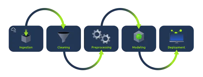
Exploring Machine Learning Pipeline #
It referens to the series of steps involved in building and deploying an ML model. The steps ensure that data flows efficiently from its raw form to predictions and insights.
A typical pipeline would include collecting data from different sources in different forms, preprocessing it and performing feature extraction from the data, splitting the data into testing and training data, and then applying Machine Learning models and predictions.
Step #0: Importing the required libraries #
We need, like in previous tasks, the following libraries:
import numpy as np
import pandas as pd
Step #1: Data Collection #
Is the process of gathering raw data from various sources to be used for ML.
The data can originate from numerous sources, like databases, text files, APIs, online repos, sensors, surveys, web scraping and much more.
The dataset used contains spam and ham (non-spam) emails.
data = pd.read_csv('emails_dataset.csv')
To review the dataset, we use Pandas DataFrames to provide a structured and tabular representation of data.
df = pd.DataFrame(data)
print(df)
Step #2: Data Preprocessing #
Refers to the techniques used to convert raw data into a clean, organised, understandable and structured format suitable for ML.
This is an essential step. Raw data is often messy, inconsistent and incomplete.
Here are some common techniques used in data preprocessing:
| Technique | Description | Use Cases |
|---|---|---|
| Cleaning | Correct errors, fill missing values, smooth noise and handle outliers. | To ensure the quality and consistency of the data. |
| Normalization | Scaling numeric data into a uniform range, typically [0,1] or [-1, 1]. | When features have different scales and we want equal contribution from all features. |
| Standardization | Rescaling data to have a mean (μ) of 0 and a standard deviation (σ) of 1 (unit variance). | When we want to ensure that the variance is uniform across all features. |
| Feature Extraction | Transforming arbitrary data such as text or images into numerical features. | To reduce the dimensionality of data and make patterns more apparent to learning algorithms. |
| Dimansionality Reduction | Reducing the number of variables under consideration by obtaining a set of principal variables. | To reduce the computational cost and improve the model’s performance by reducing noise. |
| Discretization | Transforming continuous variables into discrete ones. | To handle continuous variables and make the modle more interpretable. |
| Text preprocessing | Tokenization, stemming, lemmatization etc. to convert text to a format usable for ML algorithms. | To process and structure text data before feeding it into text analysis models. |
| Imputation | Replacing missing values with statistical values such as mean, median, mode or a constant. | To handle missing data and maintain the dataset’s integrity. |
| Feature Engineering | Creating new features or modifying existing ones to improve model performance. | To enhance the predictive power of the learning algorithms by creating features that capture more information. |
Utilizing CountVectorizer() #
ML models understand numbers and not text. To transform text into a numerical format we use CountVectorizer, a class provided by the scikit-learn python library.
This is achieved by converting text into a token (word) count matrix. It is used to prepare the data for the ML model to use and predict decisions on.
from sklearn.feature_extraction.text import CountVectorizer
vectorizer = CountVectorizer()
X = vectorizer.fit_transform(df['Message'])
print(X)
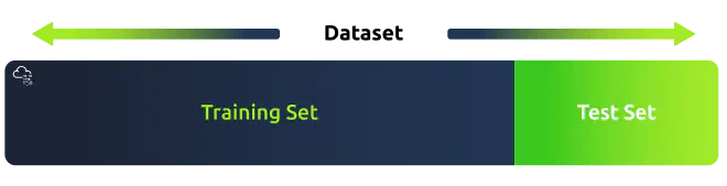
Step #3: Train/Test Split Dataset #
It’s important to test the model’s performance on unseen data. By splitting the data, we can train our model on one subset and test its performance on another.
from sklearn.model_selection import train_test_split
y = df['Classification']
X_train, X_test, y_train, y_test = train_test_split(X, y, test_size=0.2)
- X: The first argument to
train_test_splitis the feature matrixXwhich you obtained from theCountVectorizer. This matrix contains the token counts for each message in the dataset. - y: The second argument is the labels for each instance in your dataset. This indicates whether a message is spam or ham.
- test_size=0.2: This argument specifies that 20% of the dataset should be kept as the test set and the rest should be used for training.
The function then returns:
- X_train: Subset of the features to be used for training.
- X_test: Subset of the features to be used for testing.
- y_train: Corresponding labels for the X_train set.
- y_test: Corresponding labels for the y_train set.
Step #4: Model Training #
| Model | Explanation |
|---|---|
| Naive Bayes Classifier | A probabilistic classifier based on Bayes’ Theorem with an assumption of independence between features. It’s particularly suited for high-dimensional text data. |
| Support Vector Machine (SVM) | A robust classifier that finds the optimal hyperplane to separate different classes in the feature space. Works well with non-linear and high-dimensional data when used with kernel functions. |
| Logistic Regression | A statistical model that uses a logistic function to model a binary dependent variable, in this case, spam or ham. |
| Decision Trees | A model that uses a tree-like graph of decisions and their possible consequences; it’s simple to understand but can overfit if not pruned properly. |
| Random Forest | An ensemble of decision trees, typically trained with the “bagging” method to improve the predictive accuracy and control overfitting. |
| Gradient Boosting Machines (GBMs) | An ensemble learning method is building strong predictive models in a stage-wise fashion; known for outperforming random forests if tuned correctly. |
| K-Nearest Neighbors (KNN) | A non-parametric method that classifies each data point based on the majority vote of its neighbors, with the data point being assigned to the class most common among its k nearest neighbors. |
Naive Bayes Model Training #
Statistical method that uses the probability of certain words appearing in spam and non-spam emails to determine whether a new email is spam or not.
How it works:
- Let’s say we have a bunch of emails, some labelled as “spam” and other as “ham”
- The Naive Bayes algorithm learns from these emails. It looks at the words in each email and calculates how frequently each word appears in spam or ham emails. For example, words like free/win/offer/lottery might appear more in spam emails.
- The Naive Bayes algorithm calculates the probability of the email being spam based on the words it contains.
- When the model is trained with Naive Bayes and gets a new email, like “Win a free toy now!”:
- “Win” often appears in spam, so this increases the chance of the email being spam.
- “Free” is also common in spam, further increasing the spam probability.
- “Toy” might be neutral, often appearing in both spam and ham.
- After considering all the words, it calculates the overall probability of the email being spam and ham.
from sklearn.naive_bayes import MultinomialNB
clf = MultinomialNB()
clf.fit(X_train, y_train)
- X_train: Training data you want the model to learn from. It’s the token counts for each message in the training dataset, obtained from the CountVectorizer.
- y_train: These are the correct labels (“spam” or “ham”) for each message in the X_train dataset.
When we call the fit method, the MultinomialNB model goes through the data and learns patterns. This is where the training of the model happens.
When the model have been trained it can be used to make predictions on new, unseen data.
Step #5: Model Evaluation #
It’s essential to evaluate the model’s performance on the test set to gauge its predictive power.
from sklearn.metrics import classification_report
y_pred = clf.predict(X_test)
print(classification_report(y_test, y_pred))
The classification_report takes in the true labels (y_test) and the predicted labels (y_pred) and returns a text report showing the main classification metrics.
- Precision: This is the ratio of correctly predicted positive observations to the total predicted positives. The question it answers is: Of all the samples predicted as positive, how many were actually positive?
- Recall (sensitivity): The ratio of correctly predicted positive observations to all the actual positives. It answers the question: Of all the actual positive samples, how many did we predict correctly?
- F1-score: The harmonic mean of the precision and recall metrics. It gives a better measure of the incorrectly classified cases than the accuracy metric, especially when there’s an imbalance between classes.
- Support: This metric is the number of actual occurrences of the class in the specified dataset.
- Accuracy: The ratio of correctly predicted observations to the total observations.
- Macro Avg: This averages the unweighted mean per label.
- Weighted Avg: This metric averages the support-weighted mean per label.
Step #6: Testing the Model #
When we are satisfied with the performance, we can us it to classify new messages and determine if they are spam or ham.
message = vectorizer.transform(["Today's Offer! Claim ur $150 worth of discount vouchers! Text YES to 85023 now! SavaMob, member offers mobile! T Cs 08717898035. $3.00 Sub. 16 . Unsbub reply X"])
prediction = clf.predict(message)
print("The email is: ", prediction[0])
The task is now to check the emails inside test_emails.csv.
test_data = pd.read_csv("test_emails.csv")
print(test_data.head())

X_new = vectorizer.transform(test_data['Messages'])
new_predictions = clf.predict(X_new)
results_df = pd.DataFrame({'Messages': test_data['Messages'], 'Prediction': new_predictions})
print(results_df)
Questions #
- What is the key first step in the Machine Learning pipeline?
Step #1 if the pipeline.
- Which data preprocessing feature is used to create new features or modify existing ones to improve model performance?
Check the table under Step #2.
- During the data splitting step, 20% of the dataset was split for testing. What is the percentage weightage avg of precision of spam detection?
Check the output of your code when running Step #3.
- How many of the test emails are marked as spam?
Check the ouput of the last step, when running the test dataframe. Then count the number of “spam”.
- One of the emails that is detected as spam contains a secret code. What is the code?
Check the raw data for the emails marked as spam.